
In this tutorial, we will see how to easily freeze row in google sheets. Before we dive into the tutorial, let us see why we need freezing of a row.
Suppose you want to create a table whose first row contains category on the basis of which table needs to be filled. Let us take an example. Suppose you need to create a list of students with their name, father name, class, and section. You add these categories like name, father name, etc. in the first row. When you scrolled down, the first-row disappears. This creates a problem to know whether the first column is name or father name or the third column is class or section. To solve this issue, generally, rows are fixed.
How to freeze first row in google sheet
Step-1: Open the document in google sheets.
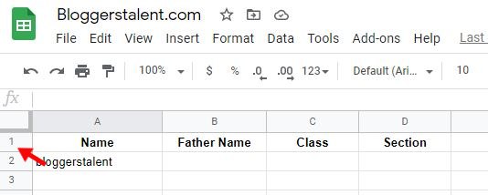
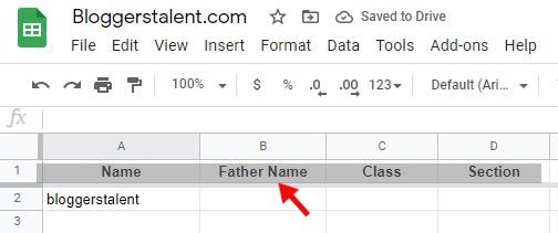
Step-2: Click on the row number 1 as shown below. This will select the entire row 1.
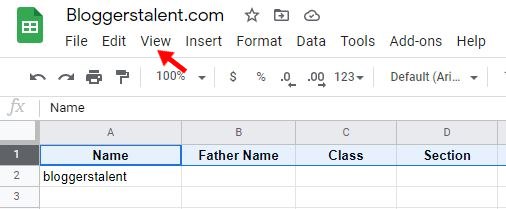
Step-3: Now click on the View option in the menubar as shown below.
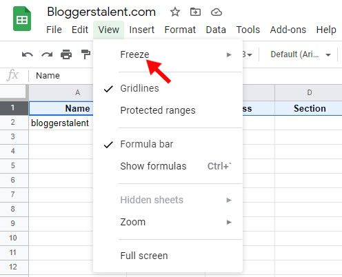
Step-4: Now click on the freeze option as shown below.
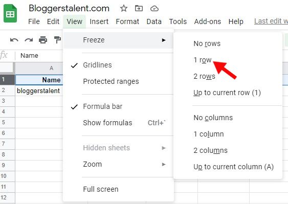
Step-5: A sidebar will open. Click on the 1 row option as shown below. This will freeze the first row.
Step-6: Here your first row is frozen. It does not move when you scroll up and down. A visible grey line appears after the first row as shown below.
I hope this tutorial on how to freeze row in Google Sheets would help you in freezing the row. If you any query, please do comment below.