
In this tutorial, we will see how can you freeze columns in google sheets. Sometimes we need freezing of a column. It becomes cumbersome if we have large data in sheets. When you scroll left to right then whole sheet slides. Hence it will hide the column one by one. Generally, we put the category in the first column. Based on that we put data into it. If we can freeze the column it becomes easy for us to know which entry belongs to which category.
How to freeze first column in google sheets
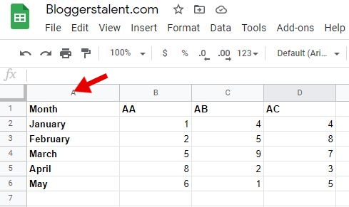
Step-1: Open the excel document in google sheets.
Step-2: Click on column number 1 as shown below. This will select the entire column 1.
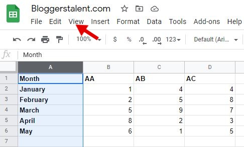
Step-3: Now click on the View option in the menubar as shown below.
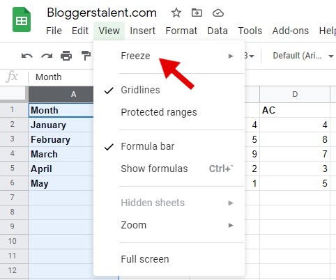
Step-4: You have to click on the Freeze option as shown below.
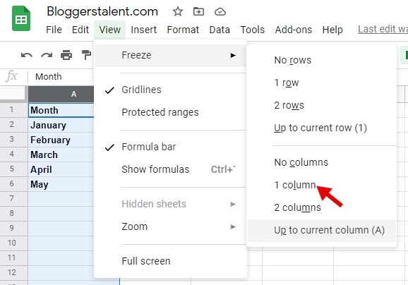
Step-5: A sidebar will open. Click on the 1 column option as shown below. This will freeze the first column.
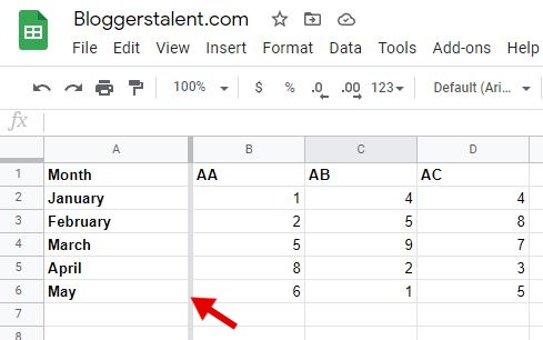
Step-6: Here your first column is frozen. It does not move when you scroll left to right or right to left. A visible grey line (as shown in the figure below) appears after the first column which shows that column is fixed.
I hope this tutorial on how to freeze columns in Google Sheets would help you in freezing the columns. You can post your query in the comments below.